
There are two easy ways to highlight every other row or column in a worksheet, which makes it much easier to read mind-numbing rows of data.
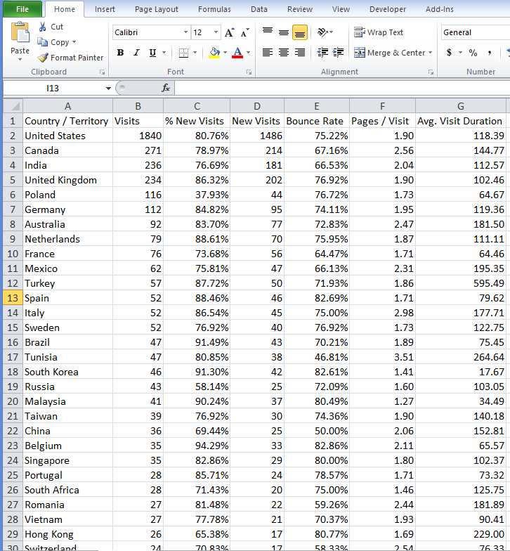 |
| Mind-Numbing hard to follow rows |
The first method is to highlight the necessary cells and find “Format As Table” on the toolbar. Choose the style of table and then select the area to be included in the table.
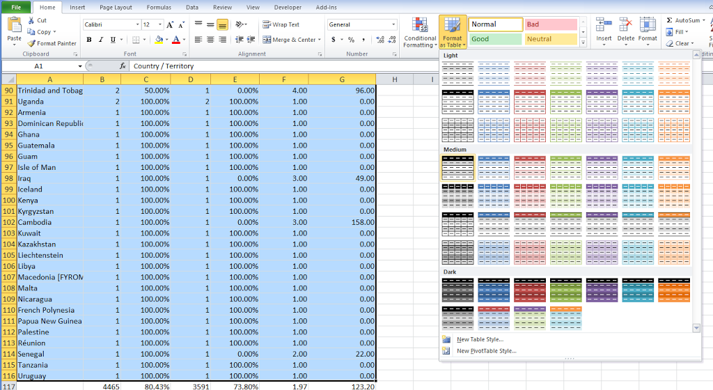 |
| Select from the endless color options |
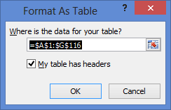 |
| Check has header to make the first row called out in a unique format |
To alter a table after it has been created highlight anywhere in it then click ‘Table Tools’ and Design subtab
When formatted as a table you can insert rows and they will automatically get the right formatting. This is helpful so that if you need to add an odd number of rows to a table you do not have to reformat the whole thing.
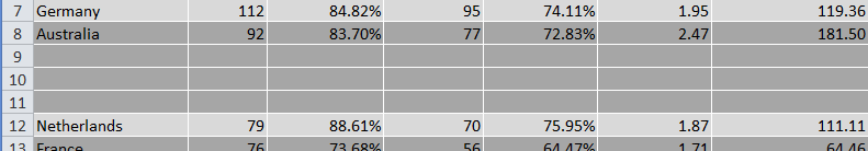 |
| Non Formatted Table – Insert rows and they do not pick up the correct alternating shading |
| When Formatted as a table a new row inserted will automatically be correctly shaded (as will all others below it) |
The second method is to use conditional formatting to highlight the rows. This can be useful if you want to highlight cells already within a table (ie. call them out as red in a sea of alternating gray), or if you simply do not want to use a table.
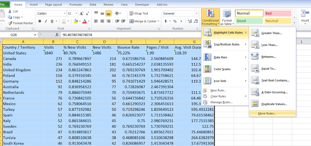
Conditional formatting can be used in a number of ways, but to highlight alternates you need to define a unique rule. Select the New Rule option from the menu.
For the rule type use a formula of “=Mod(Row(),2)=0”
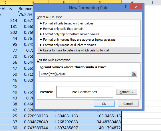
So what is this formula doing?
The equation is to check if a formula is true. Looking all the way to the right we see that =0 is what the formula is checking for truth. Mod(Number/Divisor) will find the remainder of a number divided by the divisor, then given above, it is checked to see if 0 is the remainder. Row() simply uses the row number.
So the formula takes the row value, divides by 2, and sees if the remainder is zero. Basically every even numbered row will be highlighted.
Highlight alternating ODD rows in Excel:
Take the above and change the formula to =Mod(Row(),2)=1
This forumla dives the row number by two. If there is a remainder of 1 (which there is for all even numbers) then that row becomes highlighted. Using both equations of the same range of cells you can generate individually highlighted sections within a pre-formatted table.
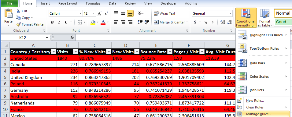
For conditional formatting it is also useful to know how to alter the conditional formatting rule.
 |
| Manage Conditional formatting rule to change the range of alternate highlights |
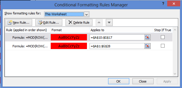 |
| Change the range of cells or resultant format of the cell of each rule individually. |
Presenting useful information in a cohesive format is one of the best uses of Excel. Knowing both of these methods can help make in decipherable data more readable